Harris corner detection

What have I been doing

This week I was officially given the task sheet for the project presentation in which I will be creating a stereo vision system. Considering this, I should probably stop procrastinating (as I did over the holidays), and finally get to finding similar objects between different images. There are many ways of finding these similar objects, however a popular method has been to find the corners of objects, as corners are typically easy to see for computers. The iconic algorithm for doing this is Harris Corner Detection, which works but is not the most optimized method. I am struggling to decide one whether to do Harris Corner Detection which is well documented and would be easy to implement or a more effective object definition algorithm. Using a corner detection algorithm presents a distinct advantage over some other form of similar point detection, as it is easier to create 3d geometry from corners than more arbitrary similar points.

Harris corner detection

Harris corner detection is fairly simple in concept. You essentially compute the brightness gradient of a small section of a black and white image. If this gradient is large enough in multiple directions (i.e. there is a drastic change in brightness), there is most likely a corner there. This operation is peformed iteratively across the entire image, while the corners are recorded as x, y pixel positions. The corner response function also returns a value that describes the likelihood of the pixel being a corner, which can be used to match similar corners across the two captured images.

Sobel Filter

The first step in harris corner detection is technically not required, but it greatly increases accuracy. A Sobel filter is applied to the image. This essentially is an estimate of the brightness gradient within a specific window translated into a new image. So each pixel of the Sobel filtered image is the gradient of its surrounding 8 pixels, which is visualized well in the below animation.

Plotke, 2013

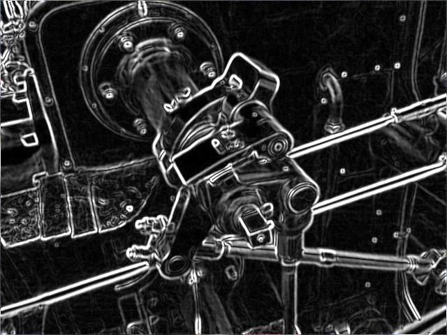
This has the effect of highlighting the edges of the image, as the pixels on an edge will have a higher gradient and therefore a higher brightness value. This can be seen in the below image where the edges are clearly brighter than the surroundings.

“Simpsons Contributer”, 2008

This gradient is calculated by convolving a preset 3x3 matrix called a kernel, and the window i.e. 3x3 matrix of pixels around the current pixel (as shown in the above animation). Convolution is a specific type of matrix multiplication which has you rotate the matrix 180 degrees, and then sum the product of each corresponding number. An example of a 3x3 convolution can be seen below. Additionally, the below image uses the same kernel that is used to find the gradient of the window in the x direction.

\[ \begin{bmatrix} 1 & 0 & -1 \\ 2 & 0 & -2 \\ 1 & 0 & -1 \end{bmatrix} \ast \begin{bmatrix} a & b & c \\ d & e & f \\ g & h & i \end{bmatrix} = (-a + c - 2d + 2f - g + i) \]

Consider A to be the image with pixel brightness values denoted by A(x,y). Also consider x, y to correspond to the x and y position of the current pixel. In this case the x and y gradient for any pixel is given by the below formula

\[ \begin{gathered} g_x = \begin{bmatrix} 1 & 0 & -1 \\ 2 & 0 & -2 \\ 1 & 0 & -1 \end{bmatrix} \ast \begin{bmatrix} A(x-1,y+1) & A(x,y+1) & A(x+1,y+1) \\ A(x-1,y) & A(x,y) & A(x+1,y) \\ A(x-1,y-1) & A(x,y-1) & A(x+1,y-1) \end{bmatrix} \\ = (-A(x-1,y+1) + A(x+1,y+1) - 2A(x-1,y) \\ + 2A(x+1,y) - A(x-1,y-1) + A(x+1,y-1)) \end{gathered} \]

\[ \begin{gathered} g_y = \begin{bmatrix} 1 & 2 & 1 \\ 0 & 0 & 0 \\ -1 & -2 & -1 \end{bmatrix} \ast \begin{bmatrix} A(x-1,y+1) & A(x,y+1) & A(x+1,y+1) \\ A(x-1,y) & A(x,y) & A(x+1,y) \\ A(x-1,y-1) & A(x,y-1) & A(x+1,y-1) \end{bmatrix} \\ = (-A(x-1,y+1) + A(x+1,y+1) - 2A(x-1,y) \\ + 2A(x+1,y) - A(x-1,y-1) + A(x+1,y-1)) \end{gathered} \]

The new image can be made iteratively with the below python code.

img = ...
# Compute the gradient in x and y direction using Sobel filters
# Image formatted (y,x)
gx = []
gy = []
for i in range(1, img.shape[0]-1):
    row_gx = []
    row_gy = []
    for j in range(1, img.shape[1]-1):
        # Compute the gradient in x and y direction using Sobel filters
        Gx = img[i-1][j+1] + 2*img[i][j+1] + img[i+1][j+1] - img[i-1][j-1] - 2*img[i][j-1] - img[i+1][j-1] 
        Gy = img[i+1][j-1] + 2*img[i+1][j] + img[i+1][j+1] - img[i-1][j-1] - 2*img[i-1][j] - img[i-1][j+1]
        row_gx.append(Gx)
        row_gy.append(Gy)
    gx.append(row_gx)
    gy.append(row_gy)

Structure tensor

The next step is calculating the structure tensor for each pixel of the filtered image. The structure tensor is a fairly complex mathematical concept, and I have not had the time to fully understand everything it does. The basic concept of a structure tensor is that it is essentially one step deeper than a regular gradient, sort of like a second derivative. Instead of providing an average value for the gradient across the entire window with respect to the x and y directions, it describes the distribution of the gradient within said window. Say for example there was a gradient value of 4 across the x axis, this value could be drastically affected by outliers as it is a mean and therefore the corner would be difficult to find within the window. When the structure tensor is made, it is possible to find these outliers to get a better idea of where the corner is located. The formula for this can be found below.

\[ \mathbf{M} = \begin{bmatrix} \sum_{(x,y)\in W}I_{x}^{2} & \sum_{(x,y)\in W}I_{y} \\ \sum_{(x,y)\in W}I_{x}I_{y} & \sum_{(x,y)\in W}I_{y}^{2} \end{bmatrix} \]

Yes I know it looks scary but when you break it down it is not that bad. The variable W reperesents the window of the image being captured so (x,y) ∈ W reperesents every pixel within that window. The summation symbol is essentially a for loop - it is saying for every pixel in the image sum a function of (x,y). In the case of the structure tensor, the function uses the partial derivative of the image with respect to x or y (Ix or Iy). This was approximated previously with the Sobel filter. So the code essentially involves looping over the Sobel filtered image, and creating a matrix on both images based only on the Sobel filtered brightness values. The python code below implements this.

A = []
for i in range(img.shape[0]-1):
    row_A = []
    for j in range(img.shape[1]-1):
        # Calculate the elements of the structure tensor
        IxIx = gx[i][j]**2
        IyIy = gy[i][j]**2
        IxIy = gx[i][j] * gy[i][j]
        row_A.append([IxIx, IxIy, IxIy, IyIy])
    A.append(row_A)

Corner response function

From this matrix, the corner response function can finally be executed. The corner response function takes the structure tensor and returns a value depicting the likelihood that the pixel is a corner. The formula for the corner response function can be seen below.

\[ R = \operatorname{det}(M) - k(\operatorname{trace}(M))^2 \]

Det or the determinant of a 2x2 matrix is found by subtracting the product of the top right to bottom left diagonal from the product of the top left to bottom right diagonal. The trace of a matrix is the sum of the top left to bottom right diagonal. Once the corner response function has been computed, a generally arbitrary threshold can be applied to filter pixels with a low certainty of being a corner. The code for the corner response function and threshold can be found below.

# Compute the determinant and trace of the structure tensor
threshold = ...
corners = []
for i in range(img.shape[0]-1):
    for j in range(img.shape[1]-1):
        # Calculate the determinant and trace of the structure tensor
        det = A[i][j][0]*A[i][j][3] - A[i][j][1]*A[i][j][2]
        trace = A[i][j][0] + A[i][j][3]
        response = det - 0.04 * trace**2 # Use the Harris corner response function
        if response > threshold:
            corners.append((response, (j,i)))

These corners can then be compared across the two images with a threshold for how close the response function must be to determine if the same corner is in both images.

Reflection

Why was this blog post so long?

I made this blog post over the word limit because it was such a huge topic that I had to explore and I wanted to create a write up that I could use to remeber harris corner detection in the future. The last time I did a project on a complex algorithm, it was perlin noise and I did not have a good explanation of it in the assignment even though I understood the algorithm to an advanced level. I focused on the implementation and not the report, which was my downfall in terms of marks. Writing this post gives me a strong foundation for the explanation I will have to make in my report, and in my presentation so I will continue to write similar reflections in future, regardless of how long they are.